Fundamentals of Linear Control:
A Concise Approach
Chapter 4: Feedback Analysis
linearcontrol.info/fundamentals
4.1 Tracking, Sensitivity, and Integral Control
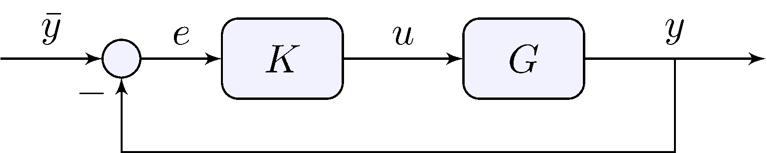
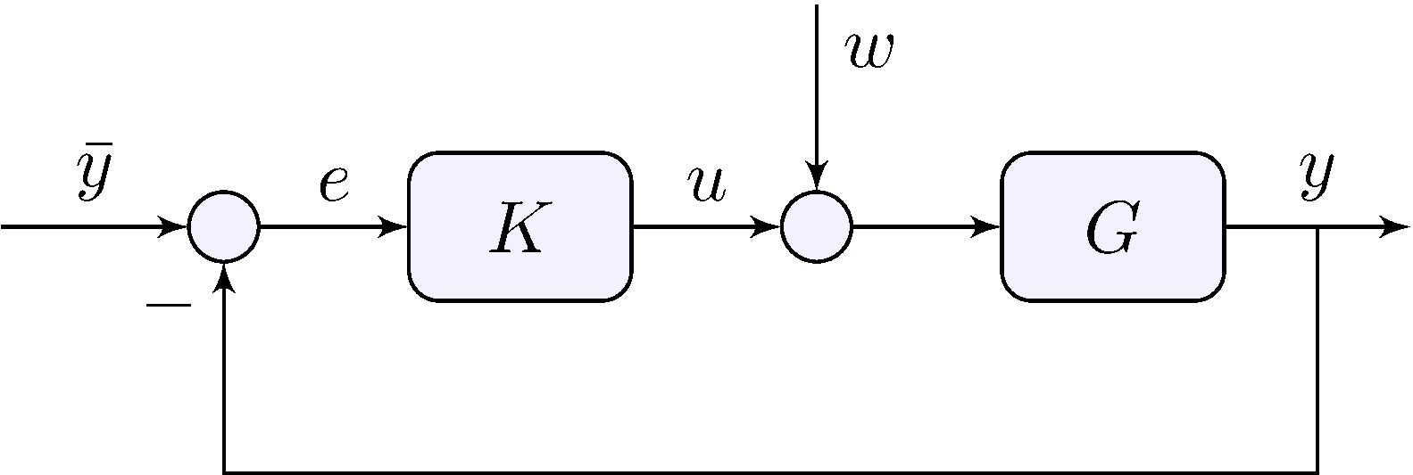
Loop relations
\[\begin{align*} Y(s) &= G(s) \, U(s), & U(s) &= K(s) \, E(s), & E(s) &= \bar{Y}(s) - Y(s) \end{align*}\]
Closed-loop sensitivity transfer-function
\[\begin{align*} E(s) &= S(s) \, \bar{Y}(s), & S(s) &= \frac{1}{1 + G(s) \, K(s)} \end{align*}\]
Short-hand notation
\[\begin{align*} e &= S \, \bar{y}, & S &= \frac{1}{1 + G \, K}, & \text{etc} \end{align*}\]
Example: car model with integral feedback
Controller
\[\begin{align*} U(s) &= \frac{K}{s} E(s) & & \implies & u(t) &= u(0) + K \int_0^t e(\tau) \, d\tau \end{align*}\]
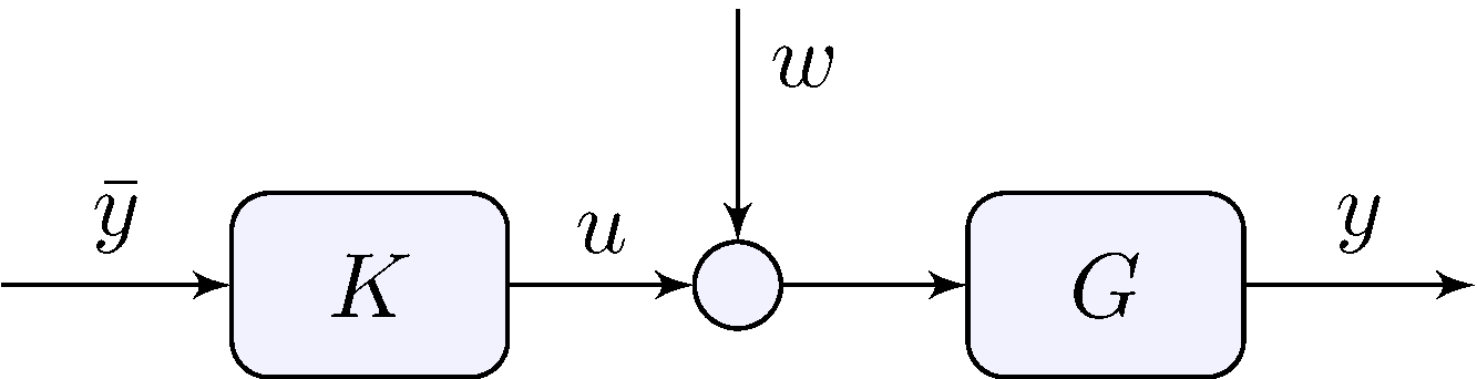
System + Controller block-diagram
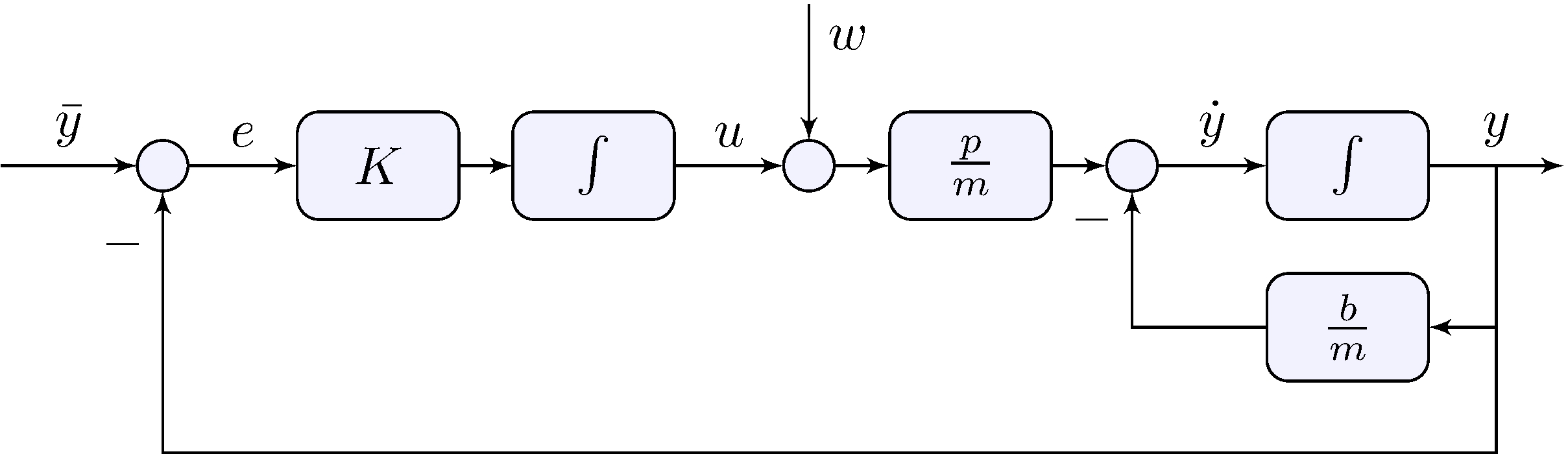
Example: car model with integral feedback
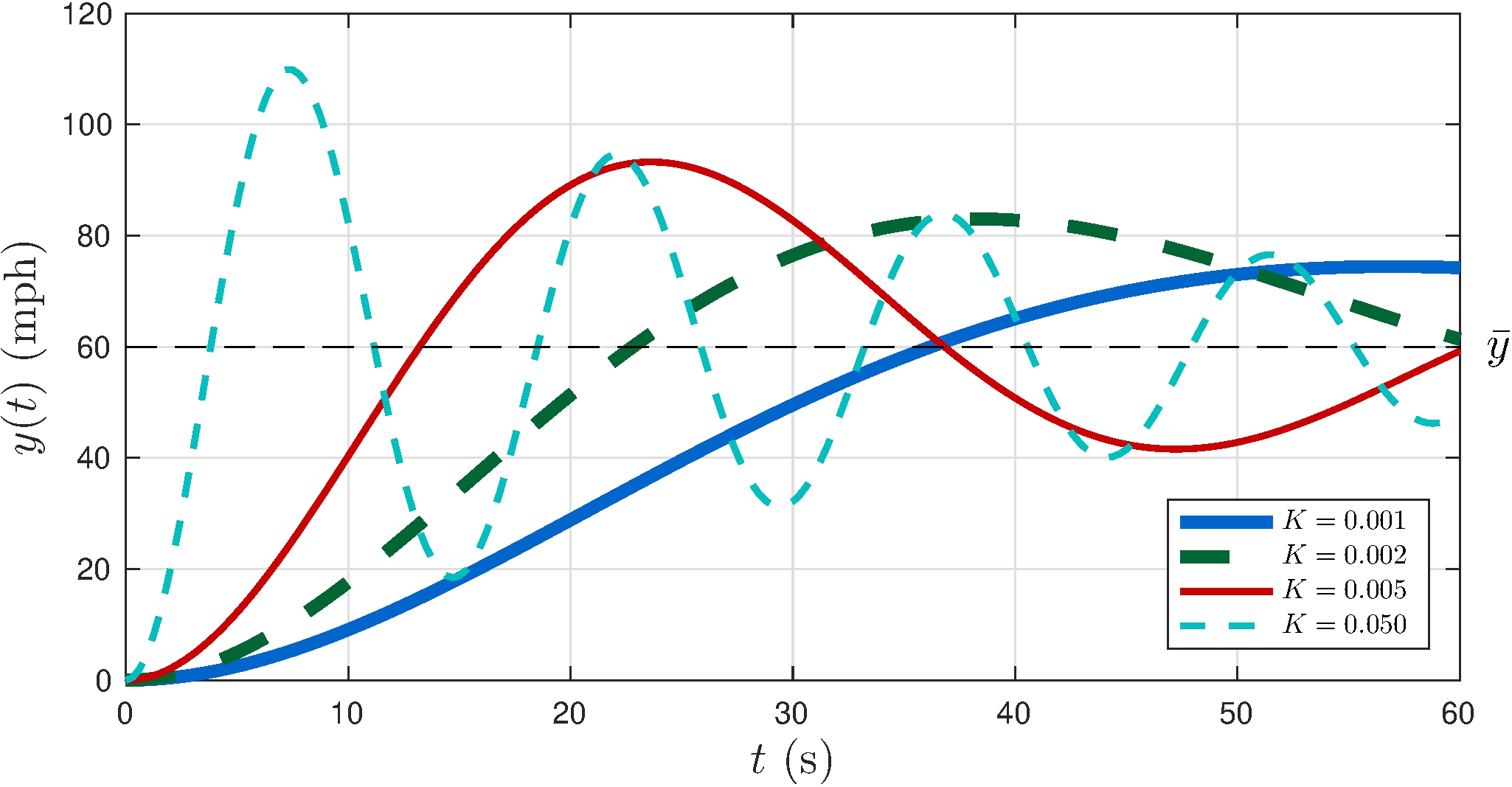
Transient response has oscilations!
Example: car model with proportional plus integral feedback
Controller
\[\begin{align*} U(s) &= \left ( K_p + \frac{K_i}{s} \right ) E(s) & & \implies & u(t) &= u(0) + K_p e(t) + K_i \int_0^t e(\tau) \, d\tau \end{align*}\]
System + Controller block-diagram
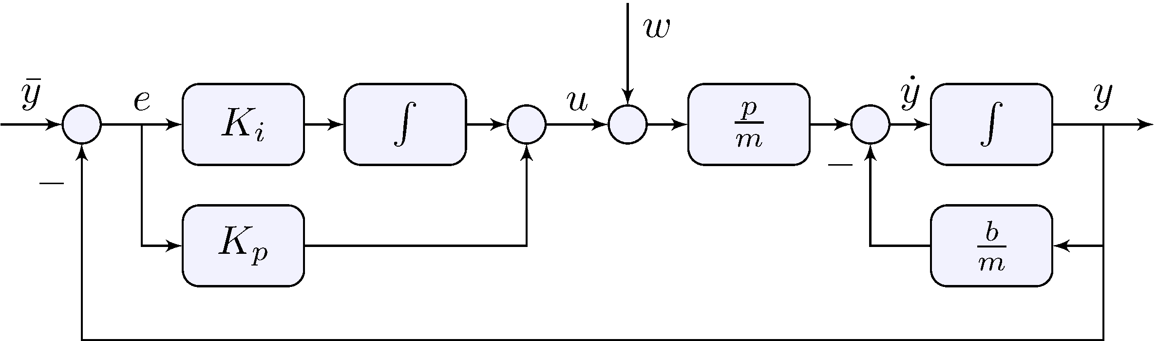
Example: car model with proportional plus integral feedback
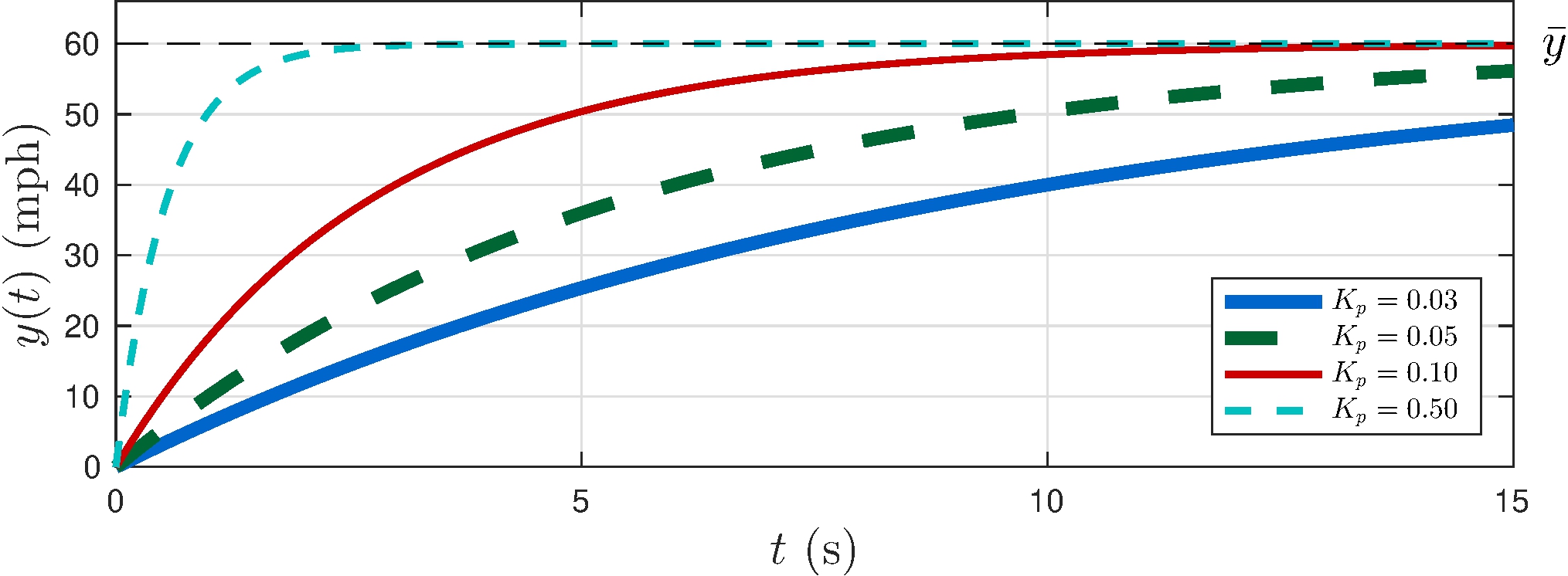
Asymptotic tracking, gone are the oscillations!
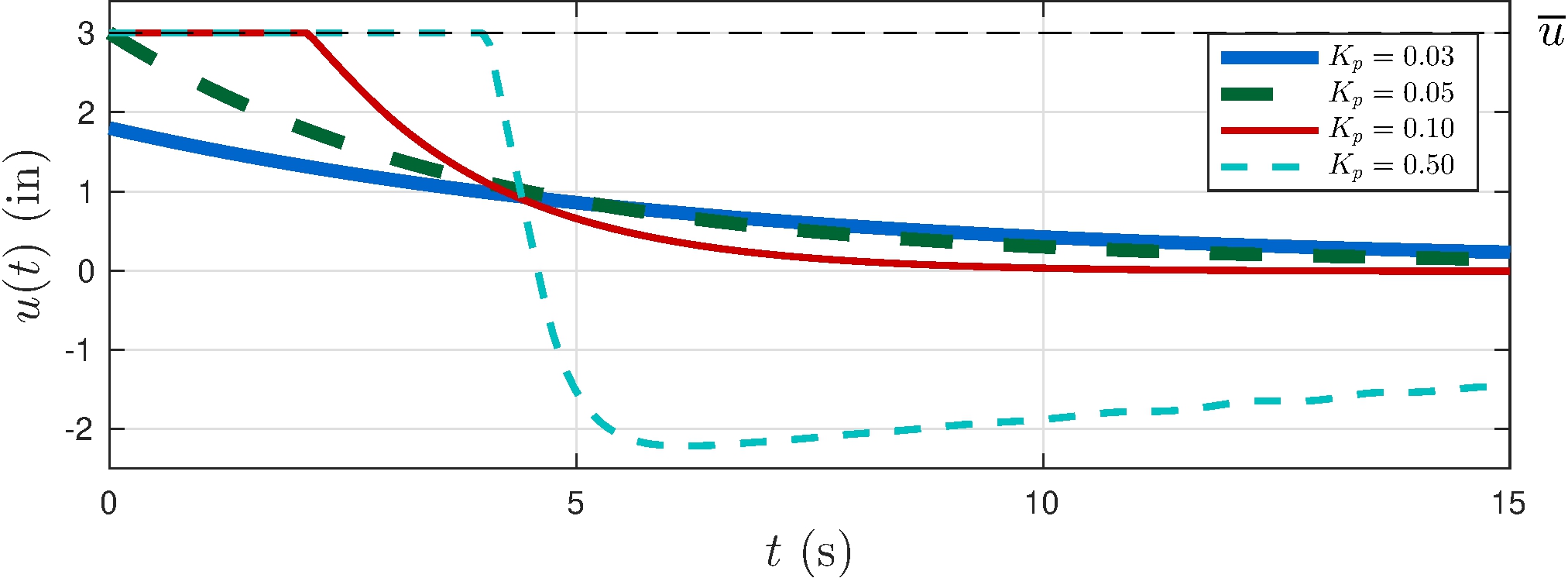
Beware of control effort: saturation occurs if \[\begin{align*} K_p > \frac{\overline{u}}{\bar{y}} = \frac{3}{60} = 0.05 \end{align*}\]
4.3 Integrator Wind-up
Example: car model with proportional plus integral feedback
Nonlinear input saturation
Output overshoots
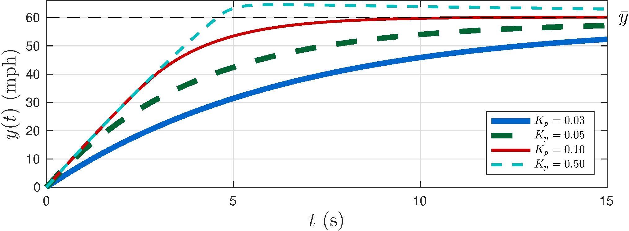
Example: car model with proportional plus integral feedback
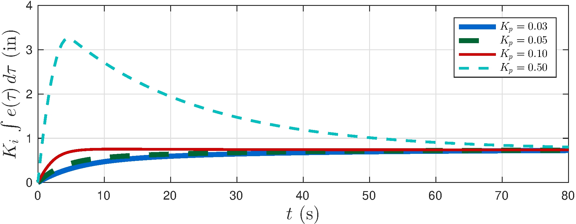
Output converges slowly
Integrator wind-up
4.4 Feedback with Disturbances
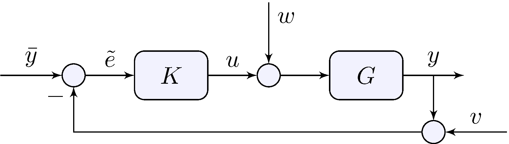
Loop relations
\[\begin{align*} y &= G \, (u + w), & u &= K \, \tilde{e}, & \tilde{e} &= \bar{y} - (y + v) \end{align*}\]
Closed-loop transfer-functions
\[\begin{align*} y &= H \, \bar{y} - H \, v + D \, w, & u &= Q \, \bar{y} - Q \, v - H \, w \end{align*}\]
Tracking error
\[\begin{align*} e &= \bar{y} - y = S \, \bar{y} + H \, v - D \, w \end{align*}\]
Beware \(\tilde{e} \neq e\)!
4.4 Feedback with Disturbances
Closed-loop transfer-functions
\[\begin{align*} y &= H \, \bar{y} - H \, v + D \, w \\ u &= Q \, \bar{y} - Q \, v - H \, w \\ e &= S \, \bar{y} + H \, v - D \, w \end{align*}\]
Gang of four
\[\begin{align*} S &= \frac{1}{1 + G K}, & D &= \frac{G}{1 + G K} & H &= \frac{G K}{1 + G K}, & Q &= \frac{K}{1 + G K} \end{align*}\]
4.4 Feedback with Disturbances
Gang of four
\[\begin{align*} S &= \frac{1}{1 + G K}, & D &= G S, & H &= G K S, & Q &= K S \end{align*}\]
- \(S\) has as zeros the poles of \(G K\)
- No pole-zero cancellations in \(G K \, \implies \, S\), \(D\), \(H\), \(Q\) have the same poles!
- Stabilizing \(S\) stabilizes all other transfer-functions
- If there are pole-zero cancellations in \(G K\) be careful and see Section 4.7
4.5 Input-Disturbance Rejection
Closed-loop transfer-functions
\[\begin{align*} e &= S \, \bar{y} - D \, w, & D &= G S = \frac{G}{1 + G K} \end{align*}\]
Lemma 4.2
Let \(S = (1 + G \, K)^{-1}\) and \(D = G S\) be asymptotically stable and \[\begin{align*} \bar{y}(t) &= \bar{y} \cos(\omega t + \phi), & w(t) &= \bar{w} \cos(\omega t + \psi) \end{align*}\] If \(K\) has a pole at \(s = j \omega\) then \(\lim_{t \rightarrow \infty} e(t) = 0\)
Proof: \(S\) and \(D\) have zeros at \(s = j \omega\)
4.5 Input-Disturbance Rejection
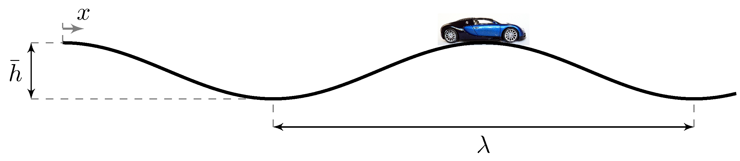
Example: car model with various feedback controllers
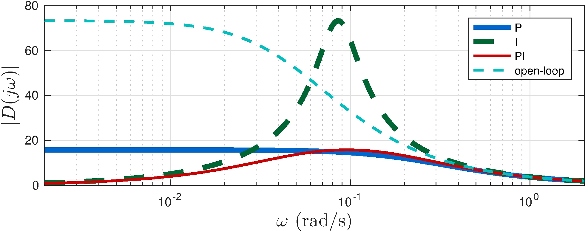
Integral controller is sensitive to disturbances at \(0.1\) rad/s
Watch out for rolling hills!
4.7 Pole-zero Cancellations and Stability
Open-loop
\[\begin{align*} G &= \frac{N_G}{D_G}, & K &= G^{-1} = \frac{D_G}{N_G}, \end{align*}\]
- \(G\) cannot be strictly proper or \(K\) will not be proper
- Even if \(G\) is proper but not strictly proper and \(K = G^{-1}\) \[\begin{align*} y &= G \, K \, \bar{y} + G w = \bar{y} + G w, & u &= K \bar{y} \end{align*}\]
- Both \(G\) and \(K\) must be stable or \(y\) or \(u\) will be unbounded
- Stabilization of unstable systems cannot be done in open-loop
4.7 Pole-zero Cancellations and Stability
Closed-loop
Internal stability if
\[\begin{align*} S, \qquad S \, G, \qquad S \, K, \qquad S \, G \, K \end{align*}\] are all asymptotically stable
Example: car model with proportional plus integral feedback
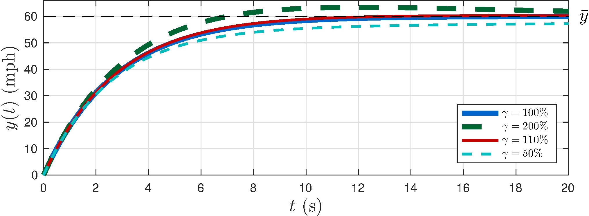
Imperfect cancellation
\[\begin{align*} K_i &= \gamma \frac{b}{m} K_p \end{align*}\]
More to come in Chapter 6