5.1 Realization of Dynamic Systems
Water tank
\[\begin{align*}
y(t) &= \frac{1}{A} \int_{0}^{t} u(\tau) \, d \tau
\end{align*}\]
\(y\): water level, \(u\): input flow
\(A\): cross-section area
Capacitor
\[\begin{align*}
v(t) &= \frac{1}{C} \int_{0}^{t} i(\tau) \, d\tau
\end{align*}\]
\(v\): voltage, \(i\): input current
\(C\): capacitance
Fly-wheel without friction
\[\begin{align*}
\omega(t) &= \frac{1}{J} \int_{0}^{t} f(\tau) \, d\tau
\end{align*}\]
\(\omega\): angular speed, \(i\): input torque
\(J\): moment of inertia
Trapezoidal integration rule
\[\begin{align*}
y(k T) - y(k T - T) &= \int_{k T - T}^{k T} u(t) \, dt \\
&\approx
\frac{T}{2} \left ( u(k T) - u(k T - T) \right )
\end{align*}\]
\(y\): integrated output, \(u\): input
\(T\): sampling period
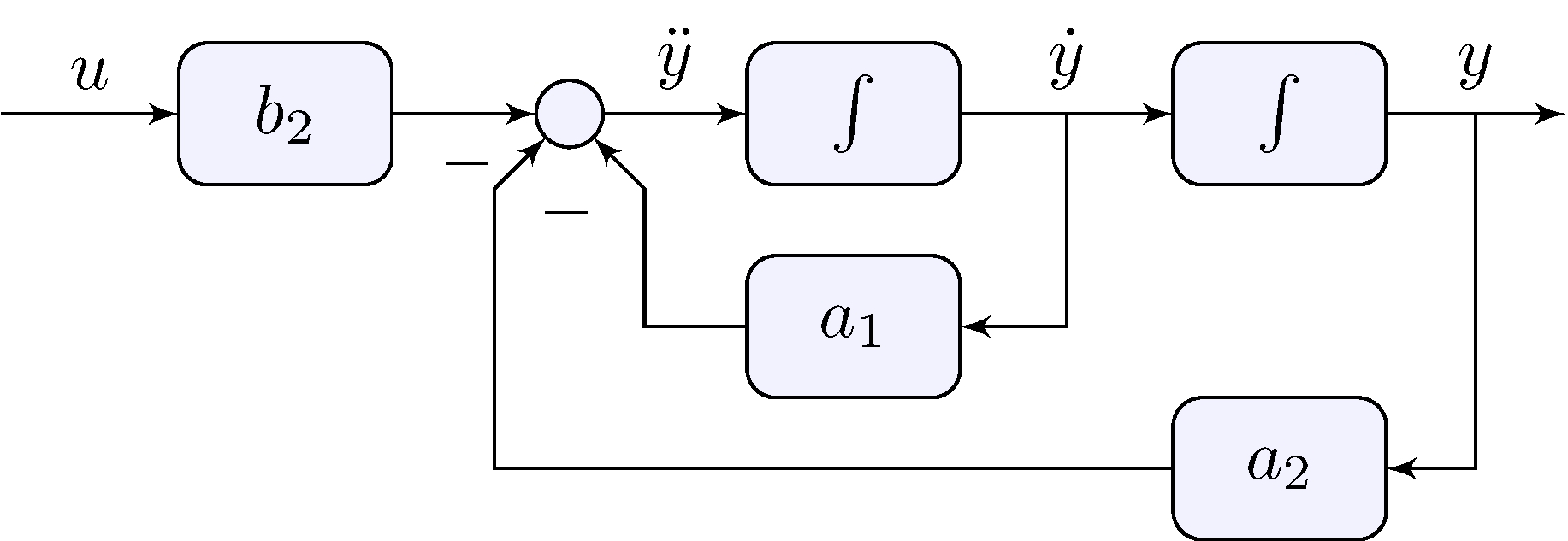
Second-order model
\[\begin{align*}
\ddot{y} + a_1 \dot{y} + a_2 \, y &= b_2 u
\end{align*}\]
Isolate highest derivative
\[\begin{align*}
\ddot{y} &= b_2 u - a_1 \dot{y} - a_2 \, y
\end{align*}\]
Block-diagram
![]()
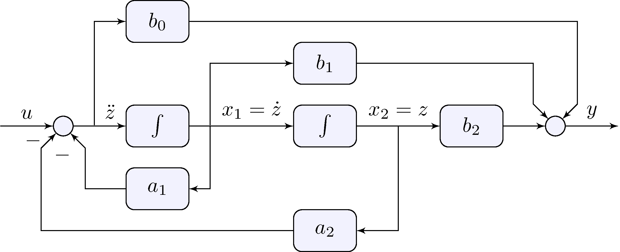
General second-order model
\[\begin{align*}
\ddot{y} + a_1 \dot{y} + a_2 \, y &= b_0 \ddot{u} + b_1 \dot{u} + b_2 u
\end{align*}\]
Linearity
\[\begin{align*}
\ddot{y} + a_1 \dot{y} + a_2 \, y &= u_0 + u_1 + u_2, &
u_0 &= b_0 \ddot{u}, &
u_1 &= b_1 \dot{u}, &
u_2 &= b_2 u
\end{align*}\] can be broken down into \[\begin{align*}
\ddot{z} + a_1 \dot{z} + a_2 \, z &= u, &
y &= b_0 \ddot{z} + b_1 \dot{z} + b_2 z
\end{align*}\]
Block-diagram
![]()
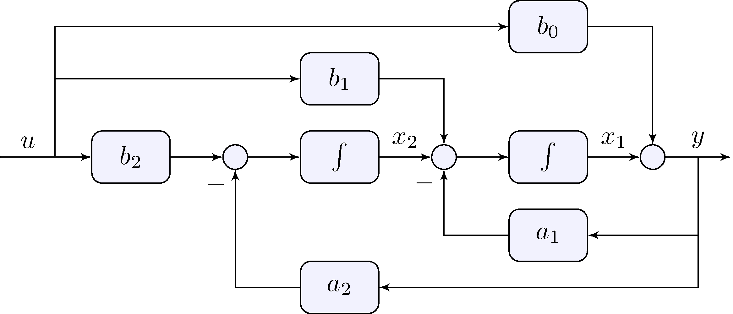
General second-order model
\[\begin{align*}
\ddot{y} + a_1 \dot{y} + a_2 \, y &= b_0 \ddot{u} + b_1 \dot{u} + b_2 u
\end{align*}\]
Isolate highest derivative
\[\begin{align*}
\ddot{y} &= b_0 \, \ddot{u} + \left ( b_1 \, \dot{u} - a_1 \,
\dot{y} \right ) + \left ( b_2 \, u - a_2 \, y \right )
\end{align*}\]
Integrate twice
\[\begin{align*}
y(t) &= b_0 u(t) + \int_{0}^{t} \left [ b_1 \, u(\tau) - a_1
\, y(\tau) + \int_{0}^{\tau} \left ( b_2 \, u(\sigma) -
a_2 \, y(\sigma) \right ) \, d\sigma \right ] d\tau
\end{align*}\]
Block-diagram
![]()
Generalizes to higher-order models
\[\begin{align*}
%\label{eq:ode}
y^{(n)}(t) + a_1 y^{(n-1)}(t) + \cdots + a_n y(t) =
b_0 u^{(m)}(t) + b_1 y^{(m-1)}(t) + \cdots + b_m u(t)
\end{align*}\]
Must be proper: \(m \leq n\)
If not proper, needs differentiator
\[\begin{align*}
y &= \dot{u}
\end{align*}\]
Impossible to realize!
Differentiator
\[\begin{align*}
u(t) &= \cos(\omega t) &
& \implies &
y_{ss}(t) &= -|\omega| \sin(\omega t)
\end{align*}\]
Unbounded amplification at high frequencies!
Integrators
\[\begin{align*}
u(t) &= \cos(\omega t) &
& \implies &
y_{ss}(t) &= \frac{1}{|\omega|} \sin(\omega t)
\end{align*}\]
Unbounded storage at low frequencies: can be dealt with in closed-loop
See book for more
5.2 State-Space Models
![]()
Integrator output = state
\[\begin{align*}
x_1 &= \dot{z}, & x_2 &= z
\end{align*}\]
\[\begin{align*}
\dot{x}_1 &= u - a_1 x_1 - a_2 x_2, &
\dot{x}_2 &= x_1
\end{align*}\]
Output
\[\begin{align*}
y &= b_0 \dot{x}_1 + b_1 x_1 + b_2 x_2
\end{align*}\]
Controllable Realization
![]()
Integrator output = state
\[\begin{align*}
x_1 &= \dot{z}, & x_2 &= z
\end{align*}\]
\[\begin{align*}
\dot{x}_1 &= u - a_1 x_1 - a_2 x_2, &
\dot{x}_2 &= x_1
\end{align*}\]
Output
\[\begin{align*}
y &= (b_1 - a_1 b_0) x_1 + (b_2 - a_2 b_0) x_2 + b_0 u
\end{align*}\]
Controllable Realization
![]()
All equations
\[\begin{align*}
\dot{x}_1 &= u - a_1 x_1 - a_2 x_2 \\
\dot{x}_2 &= x_1 \\
y &= (b_1 - a_1 b_0) x_1 + (b_2 - a_2 b_0) x_2 + b_0 u
\end{align*}\]
\[\begin{align*}
\begin{pmatrix}
\dot{x}_1 \\
\dot{x}_2
\end{pmatrix}
&=
\begin{bmatrix}
- a_1 & - a_2 \\
1 & 0
\end{bmatrix}
\begin{pmatrix}
x_1 \\
x_2
\end{pmatrix}
+
\begin{bmatrix}
1 \\ 0
\end{bmatrix}
u \\
y &=
\begin{bmatrix}
b_1 - a_1 b_0 &
b_2 - a_2 b_0
\end{bmatrix}
\begin{pmatrix}
x_1 \\
x_2
\end{pmatrix}
+
\begin{bmatrix}
b_0
\end{bmatrix}
u
\end{align*}\]
Observable Realization
![]()
Integrator output = state
\[\begin{align*}
x_1, \qquad x_2
\end{align*}\]
\[\begin{align*}
\dot{x}_1 &= b_1 u - a_1 y + x_2 \\
\dot{x}_2 &= b_2 u - a_2 y
\end{align*}\]
Output
\[\begin{align*}
y &= b_0 u + x_1
\end{align*}\]
Observable Realization
![]()
Integrator output = state
\[\begin{align*}
x_1, \qquad x_2
\end{align*}\]
\[\begin{align*}
\dot{x}_1 &= - a_1 x_1 + x_2 + (b_1 - a_1 b_0) u \\
\dot{x}_2 &= - a_2 x_1 + (b_2 - a_2 b_0) u
\end{align*}\]
Output
\[\begin{align*}
y &= b_0 u + x_1
\end{align*}\]
Observable Realization
![]()
All equations
\[\begin{align*}
\dot{x}_1 &= - a_1 x_1 + x_2 + (b_1 - a_1 b_0) u \\
\dot{x}_2 &= - a_2 x_1 + (b_2 - a_2 b_0) u \\
y &= b_0 u + x_1
\end{align*}\]
\[\begin{align*}
\begin{pmatrix}
\dot{x}_1 \\
\dot{x}_2
\end{pmatrix}
&=
\begin{bmatrix}
- a_1 & 1 \\
- a_2 & 0
\end{bmatrix}
\begin{pmatrix}
x_1 \\
x_2
\end{pmatrix}
+
\begin{bmatrix}
b_1 - a_1 b_0 \\
b_2 - a_2 b_0
\end{bmatrix}
u \\
y &=
\begin{bmatrix}
1 & 0
\end{bmatrix}
\begin{pmatrix}
x_1 \\
x_2
\end{pmatrix}
+
\begin{bmatrix}
b_0
\end{bmatrix}
u
\end{align*}\]
Second-order model
\[\begin{align*}
\ddot{y} + a_1 \dot{y} + a_2 \, y &= b_0 \ddot{u} + b_1 \dot{u} + b_2 u
\end{align*}\]
\[\begin{align*}
\begin{pmatrix}
\dot{x}_1 \\
\dot{x}_2
\end{pmatrix}
&=
\begin{bmatrix}
- a_1 & - a_2 \\
1 & 0
\end{bmatrix}
\begin{pmatrix}
x_1 \\
x_2
\end{pmatrix}
+
\begin{bmatrix}
1 \\ 0
\end{bmatrix}
u \\
y &=
\begin{bmatrix}
b_1 - a_1 b_0 &
b_2 - a_2 b_0
\end{bmatrix}
\begin{pmatrix}
x_1 \\
x_2
\end{pmatrix}
+
\begin{bmatrix}
b_0
\end{bmatrix}
u
\end{align*}\]
\[\begin{align*}
\begin{pmatrix}
\dot{x}_1 \\
\dot{x}_2
\end{pmatrix}
&=
\begin{bmatrix}
- a_1 & 1 \\
- a_2 & 0
\end{bmatrix}
\begin{pmatrix}
x_1 \\
x_2
\end{pmatrix}
+
\begin{bmatrix}
b_1 - a_1 b_0 \\
b_2 - a_2 b_0
\end{bmatrix}
u \\
y &=
\begin{bmatrix}
1 & 0
\end{bmatrix}
\begin{pmatrix}
x_1 \\
x_2
\end{pmatrix}
+
\begin{bmatrix}
b_0
\end{bmatrix}
u
\end{align*}\]
State-space model
\[\begin{align*}
\dot{x} &= A x + B u \\
y &= C x + D u
\end{align*}\]
SISO:
\(x \in \mathbb{R}^n, u \in \mathbb{R}^1, y \in \mathbb{R}^1\)
MIMO:
\(x \in \mathbb{R}^n, u \in \mathbb{R}^m, y \in \mathbb{R}^p\)
Frequency-domain
\[\begin{align*}
s X(s) - x(0^-) &= A X(s) + B U(s) &
& \implies &
X(s) &= (s I - A)^{-1} B U(s) + (s I - A)^{-1} x(0^-)
\end{align*}\]
Output
\[\begin{align*}
Y(s) &= G(s) U(s) + F(s) x(0^-)
\end{align*}\] \[\begin{align*}
G(s) &= C (s I - A)^{-1} B + D, &
F(s) &= C (s I - A)^{-1}
\end{align*}\]
State-space model
\[\begin{align*}
\dot{x} &= A x + B u \\
y &= C x + D u
\end{align*}\]
Transfer-function
\[\begin{align*}
G(s) &= C (s I - A)^{-1} B + D
\end{align*}\]
Proper
\[\begin{align*}
\lim_{|s| \rightarrow \infty} (s I - A)^{-1} &= 0 &
&\implies &
\lim_{|s| \rightarrow \infty} G(s) &= D
\end{align*}\]
Characteristic equation: roots of
\[\begin{align*}
|s I - A| = \det(s I - A) = 0,
\end{align*}\] that is eigenvalues of \(A\), are the poles of \(G(s)\)
State-space model
\[\begin{align*}
\dot{x} &= A x + B u \\
y &= C x + D u
\end{align*}\]
Matrix exponential
\[\begin{align*}
\mathcal{L}^{-1} \{ (s I - A)^{-1} \} = e^{A t}, \quad t \geq 0
\end{align*}\]
Impulse response
\[\begin{align*}
g(t) = \mathcal{L}^{-1} \{ G(s) \} =
\mathcal{L}^{-1} \{ C (s I - A)^{-1} B + D \} = C e^{A t} B + D
\delta(t), \quad t \geq 0
\end{align*}\]
State-space model
\[\begin{align*}
\dot{x} &= A x + B u \\
y &= C x + D u
\end{align*}\]
Matrix exponential
\[\begin{align*}
\mathcal{L}^{-1} \{ (s I - A)^{-1} \} = e^{A t}, \quad t \geq 0
\end{align*}\]
Response to initial condition
\[\begin{align*}
y(t) = \mathcal{L}^{-1} \{ F(s) x(0^-) \} =
\mathcal{L}^{-1} \{ C (s I - A)^{-1} x(0^-) \} = C e^{A t} x(0^-), \quad t \geq 0
\end{align*}\]
Asymptotic stability
\[\begin{align*}
\operatorname{Re}(\lambda_i(A)) &< 0 &
& \Leftrightarrow &
\lim_{t \rightarrow \infty} e^{A t} &= 0
\end{align*}\]
We say \(A\) is Hurwitz
State-space model
\[\begin{align*}
\dot{x} &= A x + B u \\
y &= C x + D u
\end{align*}\]
Matrix exponential
\[\begin{align*}
\mathcal{L}^{-1} \{ (s I - A)^{-1} \} = e^{A t}, \quad t \geq 0
\end{align*}\]
Response to initial condition
\[\begin{align*}
y(t) = \mathcal{L}^{-1} \{ F(s) x(0^-) \} =
\mathcal{L}^{-1} \{ C (s I - A)^{-1} x(0^-) \} = C e^{A t} x(0^-), \quad t \geq 0
\end{align*}\]
Asymptotic stability
If \(A\) is Hurwitz then \[\begin{align*}
\lim_{t \rightarrow \infty} x(t) = \lim_{t \rightarrow \infty} e^{A t} \, x(0^-) = 0
\quad \implies \quad
\lim_{t \rightarrow \infty} y(t) = \lim_{t \rightarrow \infty} C e^{A t} \, x(0^-) = 0
\end{align*}\]
5.4 Nonlinear Systems and Linearization
State-space nonlinear model
\[\begin{align*}
\dot{x}(t) &= f(x(t), u(t)) \\
y(t) &= g(x(t), u(t))
\end{align*}\]
Taylor series
\[\begin{align*}
f(x, u) &\approx f(\bar{x}, \bar{u}) + A (x - \bar{x}) + B (u - \bar{u}) \\
g(x, u) &\approx g(\bar{x}, \bar{u}) + C (x - \bar{x}) + D (u - \bar{u})
\end{align*}\] where \[\begin{align*}
A &= \left . \frac{\partial f}{\partial x} \right |_{{\scriptstyle
x = \bar{x} \\[-1ex] \scriptstyle u = \bar{u}}}, &
B &= \left . \frac{\partial f}{\partial u} \right |_{{\scriptstyle
x = \bar{x} \\[-1ex] \scriptstyle u = \bar{u}}}, &
C &= \left . \frac{\partial g}{\partial x} \right |_{{\scriptstyle
x = \bar{x} \\[-1ex] \scriptstyle u = \bar{u}}}, &
D &= \left . \frac{\partial g}{\partial u} \right |_{{\scriptstyle
x = \bar{x} \\[-1ex] \scriptstyle u = \bar{u}}}
\end{align*}\]
State-space nonlinear model
\[\begin{align*}
\dot{x}(t) &= f(x(t), u(t)) \\
y(t) &= g(x(t), u(t))
\end{align*}\]
Equilibrium point
\[\begin{align*}
(\bar{x}, \bar{u}) : \quad f(\bar{x}, \bar{u}) &= 0
\end{align*}\]
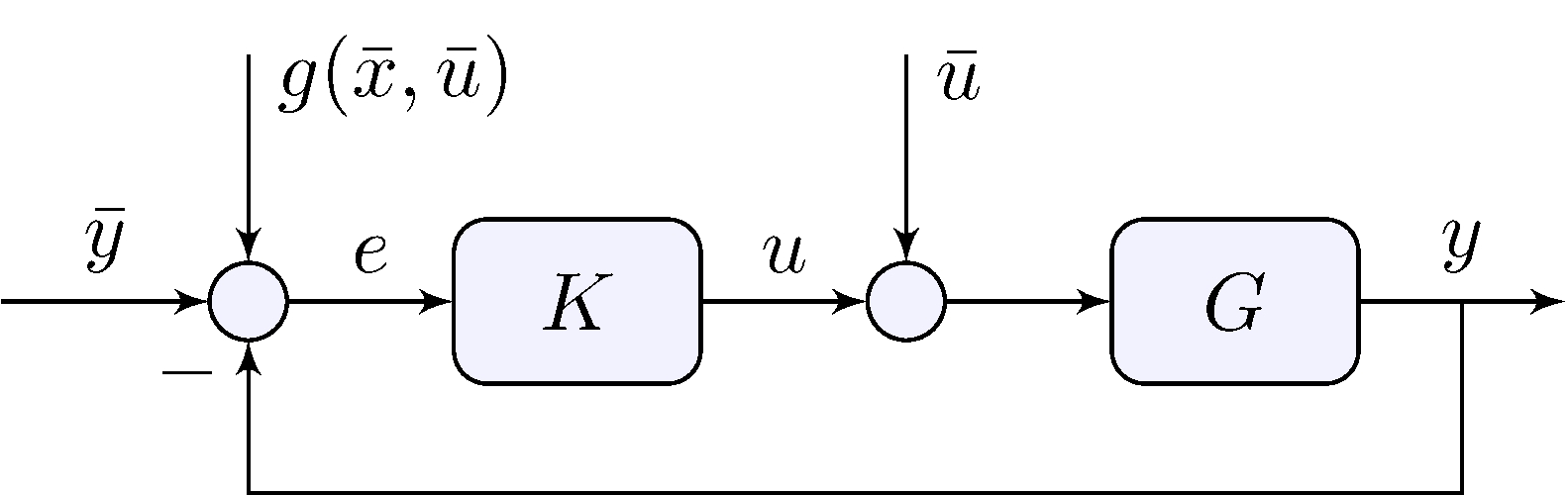
Deviations
\[\begin{align}
\tilde{x}(t) &= x(t) - \bar{x}, &
\tilde{u}(t) &= u(t) - \bar{u}, &
\tilde{y}(t) &= y(t) - g(\bar{x},\bar{u})
\end{align}\]
Taylor series
\[\begin{align*}
f(x, u) &\approx f(\bar{x}, \bar{u}) + A (x - \bar{x}) + B (u - \bar{u}) = A \tilde{x} + B \tilde{u} \\
g(x, u) &\approx g(\bar{x}, \bar{u}) + C (x - \bar{x}) + D (u - \bar{u}) = C \tilde{x} + D \tilde{u}
\end{align*}\]
State-space nonlinear model
\[\begin{align*}
\dot{x}(t) &= f(x(t), u(t)) \\
y(t) &= g(x(t), u(t))
\end{align*}\]
Equilibrium point
\[\begin{align*}
(\bar{x}, \bar{u}) : \quad f(\bar{x}, \bar{u}) &= 0
\end{align*}\]
Deviations
\[\begin{align}
\tilde{x}(t) &= x(t) - \bar{x}, &
\tilde{u}(t) &= u(t) - \bar{u}, &
\tilde{y}(t) &= y(t) - g(\bar{x},\bar{u})
\end{align}\]
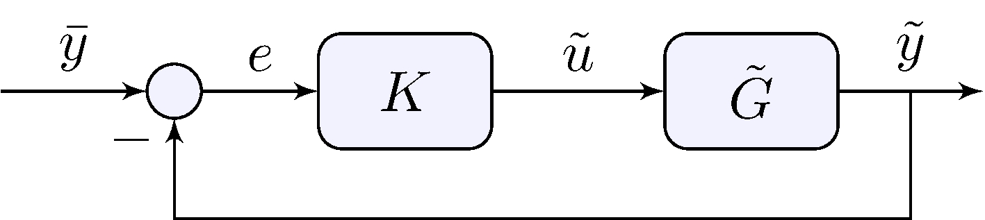
State-space linearized model
\[\begin{align*}
\dot{\tilde{x}}(t) &= A \, \tilde{x}(t) + B \, \tilde{u}(t) \\
\tilde{y}(t) &= C \, \tilde{x}(t) + D \, \tilde{u}(t)
\end{align*}\]
State-space nonlinear model
\[\begin{align*}
\dot{x}(t) &= f(x(t), u(t)) \\
y(t) &= g(x(t), u(t))
\end{align*}\]
State-space linearized model
\[\begin{align*}
\dot{\tilde{x}}(t) &= A \, \tilde{x}(t) + B \, \tilde{u}(t) \\
\tilde{y}(t) &= C \, \tilde{x}(t) + D \, \tilde{u}(t)
\end{align*}\]
Lemma 5.1 (Lyapunov)
If \(A\) is Hurwitz then there exists \(\epsilon > 0\) such that for any \(x(0)\) within \(\| x(0) - \bar{x} \| < \epsilon\) and \(u(t) = \bar{u}\) then \(\lim_{t \rightarrow \infty} x(t) \rightarrow \bar{x}\), that is \(x(t)\) converges to \(\bar{x}\)
If \(A\) has at least one eigenvalue with positive real part then there exists solutions that diverge from \(\bar{x}\)
Key points:
- Stabilitity of the linearized model implies stability of the nonlinear model “about” the equilibrium point
- No information about how large is the “region of attraction”
- Instability of the linearized model implies instability of the nonlinear model equilibrium point
- Inconclusive if eigenvalues are on the imaginary axis
- There is so much more to learn about nonlinear systems!
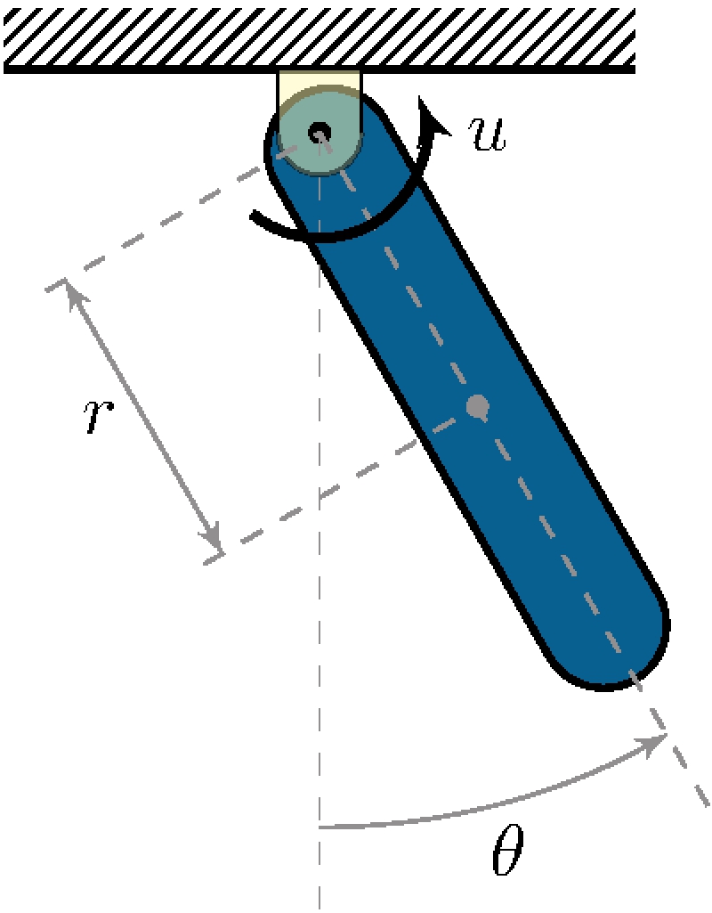
5.5 Simple Pendulum
![]()
Dynamic model
\[\begin{align*}
J_r \, \ddot{\theta} + b \, \dot{\theta} + m \, g \, r \sin
\theta &= u, &
J_r &= J + m r^2 > 0
\end{align*}\]
Nonlinear state-space model
\[\begin{align*}
x &=
\begin{pmatrix}
x_1 \\ x_2
\end{pmatrix} =
\begin{pmatrix}
\dot{\theta} \\ \theta
\end{pmatrix}, &
f(x, u) &=
\begin{pmatrix}
b_2 u - a_1 x_1 - a_2 \sin x_2 \\
x_1
\end{pmatrix}, &
g(x, u) &= x_2
\end{align*}\]
Equilibrium points (\(\bar{u} = 0\))
\[\begin{align*}
f(\bar{x}, \bar{u}) &=
\begin{pmatrix}
- a_1 \bar{x}_1 - a_2 \sin \bar{x}_2 \\
\bar{x}_1
\end{pmatrix} =
\begin{pmatrix}
0 \\ 0
\end{pmatrix} &
& \implies &
\bar{x}_1 &= 0 \quad \text{and} \quad \bar{x}_2 = k \, \pi, \quad k
\in \mathbb{Z}
\end{align*}\]
Linearization
\[\begin{align*}
\frac{\partial f}{\partial x}
&=
\begin{bmatrix}
- a_1 & - a_2 \cos x_2 \\
1 & 0
\end{bmatrix}, &
\frac{\partial f}{\partial u}
&=
\begin{bmatrix}
b_2 \\ 0
\end{bmatrix}, &
\frac{\partial g}{\partial x}
&=
\begin{bmatrix}
0 & 1
\end{bmatrix}, &
\frac{\partial g}{\partial u}
&=
\begin{bmatrix}
0
\end{bmatrix}
\end{align*}\]
About
\[\begin{align*}
(\bar{x}, \bar{u}) &= \left ( \begin{pmatrix} 0 \\ 0 \end{pmatrix}, 0
\right ): &
A_0
&=
\begin{bmatrix}
- a_1 & - a_2 \\
1 & 0
\end{bmatrix}, &
B_0
&=
\begin{bmatrix}
b_2 \\ 0
\end{bmatrix}, &
C_0
&=
\begin{bmatrix}
0 & 1
\end{bmatrix}, &
D_0
&=
\begin{bmatrix}
0
\end{bmatrix}
\end{align*}\]
Transfer-function
\[\begin{align*}
G_0(s) &= C_0 (s I - A_0)^{-1} B_0 + D_0
=
\frac{b_2}{s^2 + a_1 s + a_2}
\end{align*}\]
Equilibrium points (\(\bar{u} = 0\))
\[\begin{align*}
f(\bar{x}, \bar{u}) &=
\begin{pmatrix}
- a_1 \bar{x}_1 - a_2 \sin \bar{x}_2 \\
\bar{x}_1
\end{pmatrix} =
\begin{pmatrix}
0 \\ 0
\end{pmatrix} &
& \implies &
\bar{x}_1 &= 0 \quad \text{and} \quad \bar{x}_2 = k \, \pi, \quad k
\in \mathbb{Z}
\end{align*}\]
Linearization
\[\begin{align*}
(\bar{x}, \bar{u}) &= \left ( \begin{pmatrix} 0 \\ 0 \end{pmatrix}, 0
\right ): &
A_0
&=
\begin{bmatrix}
- a_1 & - a_2 \\
1 & 0
\end{bmatrix}, &
B_0
&=
\begin{bmatrix}
b_2 \\ 0
\end{bmatrix}, &
C_0
&=
\begin{bmatrix}
0 & 1
\end{bmatrix}, &
D_0
&=
\begin{bmatrix}
0
\end{bmatrix}
\end{align*}\]
Transfer-function
\[\begin{align*}
G_0(s) &= C_0 (s I - A_0)^{-1} B_0 + D_0
=
\frac{b_2}{s^2 + a_1 s + a_2}
\end{align*}\] If \(a_1 > 0\) and \(a_2 > 0\) then \(A_0\) is Hurwitz, \(G_0\) is asymptotically stable
Equilibrium points (\(\bar{u} = 0\))
\[\begin{align*}
f(\bar{x}, \bar{u}) &=
\begin{pmatrix}
- a_1 \bar{x}_1 - a_2 \sin \bar{x}_2 \\
\bar{x}_1
\end{pmatrix} =
\begin{pmatrix}
0 \\ 0
\end{pmatrix} &
& \implies &
\bar{x}_1 &= 0 \quad \text{and} \quad \bar{x}_2 = k \, \pi, \quad k
\in \mathbb{Z}
\end{align*}\]
Linearization
\[\begin{align*}
\frac{\partial f}{\partial x}
&=
\begin{bmatrix}
- a_1 & - a_2 \cos x_2 \\
1 & 0
\end{bmatrix}, &
\frac{\partial f}{\partial u}
&=
\begin{bmatrix}
b_2 \\ 0
\end{bmatrix}, &
\frac{\partial g}{\partial x}
&=
\begin{bmatrix}
0 & 1
\end{bmatrix}, &
\frac{\partial g}{\partial u}
&=
\begin{bmatrix}
0
\end{bmatrix}
\end{align*}\]
About
\[\begin{align*}
(\bar{x}, \bar{u}) &= \left ( \begin{pmatrix} 0
\\ \pi \end{pmatrix}, 0 \right ): &
A_\pi
&=
\begin{bmatrix}
- a_1 & a_2 \\
1 & 0
\end{bmatrix}, &
B_\pi
&=
\begin{bmatrix}
b_2 \\ 0
\end{bmatrix}, &
C_\pi
&=
\begin{bmatrix}
0 & 1
\end{bmatrix}, &
D_\pi
&=
\begin{bmatrix}
0
\end{bmatrix}
\end{align*}\]
Transfer-function
\[\begin{align*}
G_\pi(s) &= C_\pi (s I - A_\pi)^{-1} B_\pi + D_\pi
=
\frac{b_2}{s^2 + a_1 s - a_2}
\end{align*}\]
Equilibrium points (\(\bar{u} = 0\))
\[\begin{align*}
f(\bar{x}, \bar{u}) &=
\begin{pmatrix}
- a_1 \bar{x}_1 - a_2 \sin \bar{x}_2 \\
\bar{x}_1
\end{pmatrix} =
\begin{pmatrix}
0 \\ 0
\end{pmatrix} &
& \implies &
\bar{x}_1 &= 0 \quad \text{and} \quad \bar{x}_2 = k \, \pi, \quad k
\in \mathbb{Z}
\end{align*}\]
Linearization
\[\begin{align*}
(\bar{x}, \bar{u}) &= \left ( \begin{pmatrix} 0
\\ \pi \end{pmatrix}, 0 \right ): &
A_\pi
&=
\begin{bmatrix}
- a_1 & a_2 \\
1 & 0
\end{bmatrix}, &
B_\pi
&=
\begin{bmatrix}
b_2 \\ 0
\end{bmatrix}, &
C_\pi
&=
\begin{bmatrix}
0 & 1
\end{bmatrix}, &
D_\pi
&=
\begin{bmatrix}
0
\end{bmatrix}
\end{align*}\]
Transfer-function
\[\begin{align*}
G_\pi(s) &= C_\pi (s I - A_\pi)^{-1} B_\pi + D_\pi
=
\frac{b_2}{s^2 + a_1 s - a_2}
\end{align*}\] If \(a_1 > 0\) and \(a_2 > 0\) then \(A_\pi\) is not Hurwitz, \(G_\pi\) is unstable
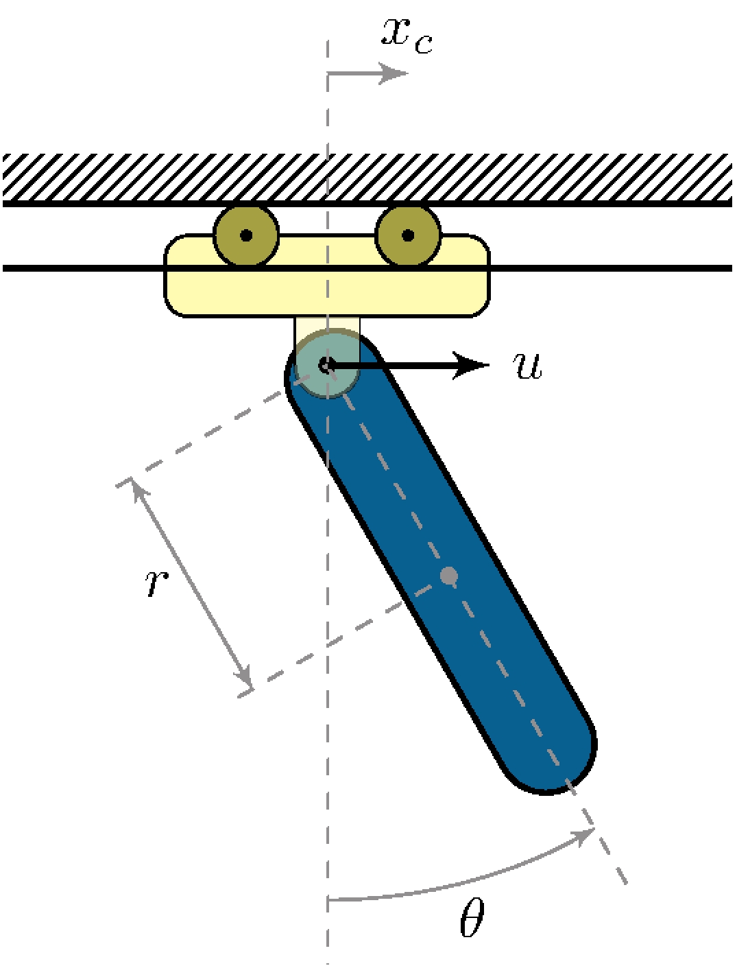
5.6 Pendulum in a Cart
Dynamic model
\[\begin{align*}
(J_p + m_p \, r^2) \ddot{\theta} + m_p \, r \, \ddot{x}_c \cos \theta
+ b_p \, \dot{\theta} + m_p \, g \, r \sin \theta &= 0 \\
m_p \, r \, \ddot{\theta} \cos \theta + (m_p + m_c) \, \ddot{x}_c +
b_c \, \dot{x}_c - m_p \, r \, \dot{\theta}^2 \sin \theta &= u
\end{align*}\]
Second-order vector differential equation
\[\begin{align*}
M(q) \, \ddot{q} + F(q, \dot{q}) &= G u, &
q &=
\begin{pmatrix}
\theta \\
x_c
\end{pmatrix}
\end{align*}\] \[\begin{align*}
M(q) &=
\begin{bmatrix}
J_p + m_p \, r^2 & m_p \, r \cos q_1 \\
m_p \, r \cos q_1 & m_p + m_c
\end{bmatrix}, &
F(q,\dot{q}) &=
\begin{pmatrix}
b_p \dot{q}_1 + m_p \, g \, r \sin q_1 \\
b_c \dot{q}_2 - m_p \, r \, \dot{q}_1^2 \sin q_1
\end{pmatrix}, &
G &=
\begin{pmatrix}
0 \\ 1
\end{pmatrix}
\end{align*}\]
Nonlinear state-space model
\[\begin{align*}
x &=
\begin{pmatrix}
q \\
\dot{q}
\end{pmatrix}, &
f(x,u) &= f(q,\dot{q},u) = \begin{pmatrix} \dot{q} \\ M^{-1}(q) \left[ G
u - F(q, \dot{q}) \right]
\end{pmatrix}
\end{align*}\]
Simplified nonlinear state-space model
\[\begin{align*}
x &=
\begin{pmatrix}
\theta \\
\dot{\theta} \\
\dot{x}_c
\end{pmatrix}, &
f(x,u) &= %f(\theta,\dot{\theta},\dot{x}_c,u) =
\begin{pmatrix}
\dot{x_1} \\ M^{-1}(x_1) \left[ G u - F(x) \right]
\end{pmatrix}
\end{align*}\]
Equilibrium points (\(\bar{u} = 0\))
\[\begin{align*}
\bar{x}_1 &= \bar{q}_1 = k \pi, \quad k \in \mathbb{Z}, &
\bar{x}_2 = \bar{x}_3 &= \bar{\dot{q}}_1 = \bar{\dot{q}}_2 = 0
\end{align*}\]
Linearization about \(\bar{x}_1 = 0\)
\[\begin{align*}
A_0 &= \frac{1}{J}
\begin{bmatrix}
0 & J & 0 \\
% 0 & 0 & 0 & J \\
-g \, m_r \, r & {-b_p \, m_r}/{m_p} & b_c \, r \\
g \, m_p \, r^2 & b_p \, r & {-b_c J_r}/{m_p} \\
\end{bmatrix}\!\!, &
B_0 &=
\frac{1}{J}
\begin{bmatrix}
0 \\ %0 \\
-r \\ {J_r}/{m_p}
\end{bmatrix}
\end{align*}\]
\[\begin{align*}
J_r &= J_p + m_p r^2 > 0, &
m_r &= m_p + m_c > 0, &
J &= J_r \frac{m_r}{m_p} - m_p r^2 > 0
\end{align*}\]
Without damping (\(b_c = b_p = 0)\)
\[\begin{align*}
\text{Eigenvalues of } A_0 &: &
& 0, &
& j \sqrt{g (m_p + m_c) r}, &
& -j \sqrt{g (m_p + m_c) r}
\end{align*}\]
Oscillator
Equilibrium points (\(\bar{u} = 0\))
\[\begin{align*}
\bar{x}_1 &= \bar{q}_1 = k \pi, \quad k \in \mathbb{Z}, &
\bar{x}_2 = \bar{x}_3 &= \bar{\dot{q}}_1 = \bar{\dot{q}}_2 = 0
\end{align*}\]
Linearization about \(\bar{x}_1 = \pi\)
\[\begin{align*}
A_\pi &= \frac{1}{J}
\begin{bmatrix}
0 & J & 0 \\
% 0 & 0 & 0 & J \\
g \, m_r \, r & {-b_p \, m_r}/{m_p} & - b_c \, r \\
g \, m_p \, r^2 & - b_p \, r & {-b_c J_r}/{m_p} \\
\end{bmatrix}\!\!, &
B_\pi &=
\frac{1}{J}
\begin{bmatrix}
0 \\ r \\ {J_r}/{m_p}
\end{bmatrix}
\end{align*}\]
\[\begin{align*}
J_r &= J_p + m_p r^2 > 0, &
m_r &= m_p + m_c > 0, &
J &= J_r \frac{m_r}{m_p} - m_p r^2 > 0
\end{align*}\]
Without damping (\(b_c = b_p = 0)\)
\[\begin{align*}
\text{Eigenvalues of } A_\pi &: &
& 0, &
& \sqrt{g (m_t + m_c) r}, &
& -\sqrt{g (m_t + m_c) r}
\end{align*}\]
Unstable