Step-by-step Bode plot example. Part IV

We continue our saga of hand sketches of the straight-line approximations for the magnitude and phase of Bode plot diagrams (Section 7.1). This time we consider a non-minimum phase system with a pole at the origin. See Part I, Part II and Part III, for simpler examples.

In this post we consider the third-order non-minimum phase transfer-function with a pole at the origin:

$$G(s) = \frac{s+2}{s(s^2-9s -10)}.$$

The only difference from the transfer-function from Part III is the additional pole at the origin. After factoring and normalizing

$$G(s) = \frac{-2}{10} \frac{1 + s/2}{s(1 + s)(1 – s/10)}.$$

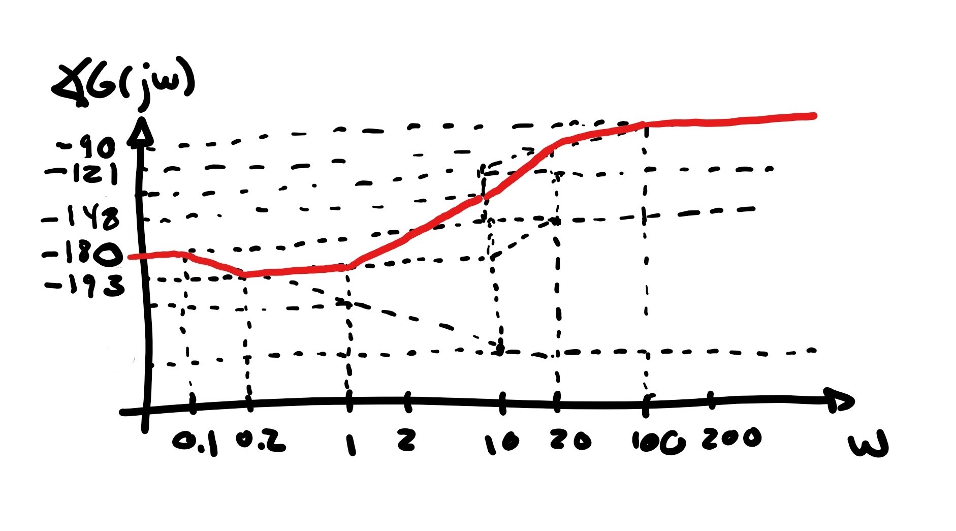
Because the effect of a pole at the origin is to add a constant $-90^\circ$ to the phase one would expect that simply shifting the diagram obtained at the end of Part III by $-90^\circ$ would suffice. This would bring the starting phase to $-270^\circ$ and the final phase to $-180^\circ$. As it turns out, the “correct” answer here is to add $360-90=270^\circ$ as opposed to subtract $90^\circ$, which leads to an initial phase of $90^\circ$ and a final phase of $180^\circ$ as in the next diagram:

The reason why we maintain that this is the “most correct” answer is that, as we will discuss in a future post in more detail, this is the answer that is most compatible with the corresponding Nyquist diagram (Section 7.6). If you do not understand why, no worries, Matlab does not seem to understand it either and also gives you the “wrong” diagram!

Now for the magnitude, start by recalling that a pole at zero implies a constant slope of $-20$dB/decade throughout the entire plot. To find out at what point we can anchor the slope we consider any $\omega$ for which no pole or zero has contributed any slope yet. In this case we can take $\omega=1$ and evaluate

$$20 \log_{10} \left |\frac{2}{10}\frac{1}{j 1}\right|\approx -13\text{dB}.$$

This leads to the red line sketch as in the next figure:

At $\omega = 1$ the pole at $s = -1$ starts contributing $-20$dB/decade to total $-40$dB/decade. This slopes lasts until the next zero at $s = -2$ starts contributing at $\omega =2$. At that point the magnitude is approximately

$$-13-40\log_{10}(2/1) \approx -13 \,- 12 = 25\text{dB}$$

leading to the sketch:

At $\omega=2$, the zero at $s = -2$ contributes $+20$db/decade, which brings the current slope to $-20$dB/decade up until $\omega = 10$ with a magnitude of approximately

$$ -25-20\log_{10}(10/2) \approx -25 – 14 = -39\text{dB}$$

as in the sketch:

At $\omega=10$ the next pole at $s=-10$ adds $-20$dB/decade to bring the current slope back to $-40$db/decade. This leads to a magnitude of

$$ -39-40\log_{10}(100/10) = -79\text{dB}$$

at $\omega=100$ and the final sketch:

Note that we do not need to consider the effect of the gain $-2/10$ because it was already considered when we anchored the pole at the origin back in the first step.